Director ratings

IMDB ratings: Differences between directors
We have a dataset containing a few thousand movies and their IMBD ratings. We want to explore whether movies directed by Steven Spielberg and Tim Burton are rated the same.
We have loaded the data and shown a glimpse of it below.
movies <- read_csv(here::here('data/movies.csv'))
glimpse(movies)
## Rows: 2,961
## Columns: 11
## $ title <chr> "Avatar", "Titanic", "Jurassic World", "The Avenge…
## $ genre <chr> "Action", "Drama", "Action", "Action", "Action", "…
## $ director <chr> "James Cameron", "James Cameron", "Colin Trevorrow…
## $ year <dbl> 2009, 1997, 2015, 2012, 2008, 1999, 1977, 2015, 20…
## $ duration <dbl> 178, 194, 124, 173, 152, 136, 125, 141, 164, 93, 1…
## $ gross <dbl> 7.61e+08, 6.59e+08, 6.52e+08, 6.23e+08, 5.33e+08, …
## $ budget <dbl> 2.37e+08, 2.00e+08, 1.50e+08, 2.20e+08, 1.85e+08, …
## $ cast_facebook_likes <dbl> 4834, 45223, 8458, 87697, 57802, 37723, 13485, 920…
## $ votes <dbl> 886204, 793059, 418214, 995415, 1676169, 534658, 9…
## $ reviews <dbl> 3777, 2843, 1934, 2425, 5312, 3917, 1752, 1752, 35…
## $ rating <dbl> 7.9, 7.7, 7.0, 8.1, 9.0, 6.5, 8.7, 7.5, 8.5, 7.2, …To start assessing this, we create a dataframe with the 95% confidence interval for the mean of the rating for each of the directors, using the t-statistic. Then we plot the confidence intervals on the same graph to see if they overlap a lot.
chosen_directors <- c('Tim Burton','Steven Spielberg')

# summarising the ratings of both of the directors
directors <- movies %>%
  filter(director %in% chosen_directors) %>%
  group_by(director) %>%
  summarise(mean_rating = mean(rating),
            sd_rating = sd(rating),
            count = n(),
            t_critical = qt(0.975, count-1),
            se_rating = sd_rating/sqrt(count),
            margin_of_error = t_critical * se_rating,
            lower = mean_rating - margin_of_error,
            upper = mean_rating + margin_of_error) %>%
  mutate(labels = round(mean_rating, 2))

skim(directors)| Name | directors |
| Number of rows | 2 |
| Number of columns | 10 |
| _______________________ | |
| Column type frequency: | |
| character | 1 |
| numeric | 9 |
| ________________________ | |
| Group variables | None |
Variable type: character
| skim_variable | n_missing | complete_rate | min | max | empty | n_unique | whitespace |
|---|---|---|---|---|---|---|---|
| director | 0 | 1 | 10 | 16 | 0 | 2 | 0 |
Variable type: numeric
| skim_variable | n_missing | complete_rate | mean | sd | p0 | p25 | p50 | p75 | p100 | hist |
|---|---|---|---|---|---|---|---|---|---|---|
| mean_rating | 0 | 1 | 7.25 | 0.45 | 6.93 | 7.09 | 7.25 | 7.41 | 7.57 | ▇▁▁▁▇ |
| sd_rating | 0 | 1 | 0.72 | 0.04 | 0.69 | 0.71 | 0.72 | 0.74 | 0.75 | ▇▁▁▁▇ |
| count | 0 | 1 | 19.50 | 4.95 | 16.00 | 17.75 | 19.50 | 21.25 | 23.00 | ▇▁▁▁▇ |
| t_critical | 0 | 1 | 2.10 | 0.04 | 2.07 | 2.09 | 2.10 | 2.12 | 2.13 | ▇▁▁▁▇ |
| se_rating | 0 | 1 | 0.17 | 0.03 | 0.14 | 0.16 | 0.17 | 0.18 | 0.19 | ▇▁▁▁▇ |
| margin_of_error | 0 | 1 | 0.35 | 0.07 | 0.30 | 0.33 | 0.35 | 0.37 | 0.40 | ▇▁▁▁▇ |
| lower | 0 | 1 | 6.90 | 0.52 | 6.53 | 6.72 | 6.90 | 7.09 | 7.27 | ▇▁▁▁▇ |
| upper | 0 | 1 | 7.60 | 0.38 | 7.33 | 7.47 | 7.60 | 7.74 | 7.87 | ▇▁▁▁▇ |
| labels | 0 | 1 | 7.25 | 0.45 | 6.93 | 7.09 | 7.25 | 7.41 | 7.57 | ▇▁▁▁▇ |
# making a plot containing the confidence intervals of the mean of the ratings of each of the directors
ggplot(data = directors) +
  aes(y = director) +
  geom_errorbarh(aes(xmin = lower, xmax = upper, color = director), size = 2, height = 0.1) +
  geom_point(aes(x = mean_rating, color = director), size = 5) +
  geom_rect(aes(xmin = 7.27, xmax = 7.33, ymin=0,ymax=3), fill = 'grey70', alpha=0.5) +
  geom_text(aes(x = mean_rating, label = labels), vjust = 0, nudge_y = 0.05, overlap=FALSE) +
  labs(
    title = 'Do Tim Burton and Steven Spielberg have the same mean IMDB rating?',
    subtitle = '95% confidence intervals overlap',
    x = 'Rating',
    y = NULL
  ) +
  theme_minimal()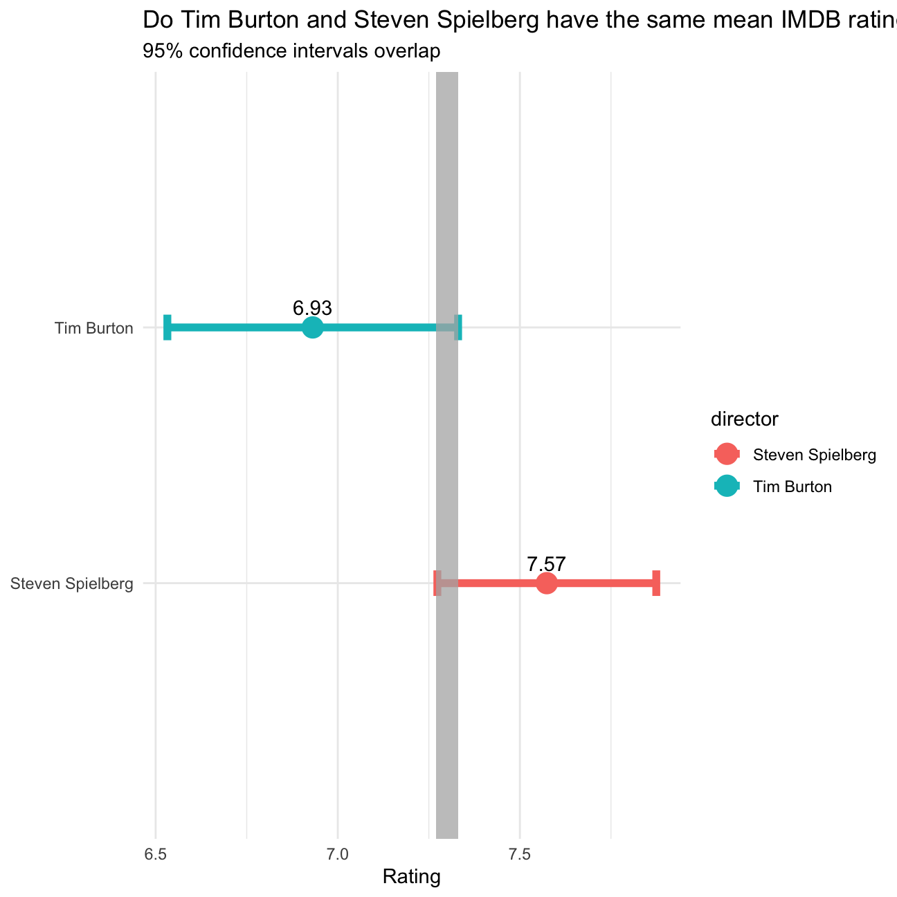
Seeing that the two intervals overalp in the grey highlighted area, we need to also conduct a statistical test to see if the means are statistically significantly different. For this, we run a t-test and use the infer package to bootstrap the data as well.
Our null hypothesis is that the means of the ratings of their films is the same. The alternative hypothesis is that there is a difference between the means of the ratings of Tim Burtons and Steven Spielbergs films. We will be using the t-statistic for the difference between the means. We are looking for a p-value smaller than 0.05 or a t-statistic bigger than 1.75 or smaller than -1.75 (based on df = 15 and p = 0.05). We have chosen the degrees of freedom as the smallest count - 1, which was 16 for Tim Burton.
df_directors <- movies  %>%
  filter(director %in% chosen_directors)

t.test(rating ~ director, data = df_directors)
##
## Welch Two Sample t-test
##
## data: rating by director
## t = 3, df = 31, p-value = 0.01
## alternative hypothesis: true difference in means between group Steven Spielberg and group Tim Burton is not equal to 0
## 95 percent confidence interval:
## 0.16 1.13
## sample estimates:
## mean in group Steven Spielberg mean in group Tim Burton
## 7.57 6.93directors_infer <- df_directors %>%
# specify variables
specify(rating ~ director) %>%
# assume independence, i.e, there is no difference
hypothesize(null = "independence") %>%
# generate 1000 reps, of type "permute"
generate(reps = 1000, type = "permute") %>%
# calculate statistic of difference, namely "diff in means"
calculate(stat = "diff in means", order = chosen_directors)directors_infer %>%
get_p_value(obs_stat = directors_infer, direction = "two-sided")## # A tibble: 1 × 1
## p_value
## <dbl>
## 1 0According to both the t.test and the bootstrapped result, there is a signficant difference in the ratings of the movies of Tim Burton and Steven Spielberg. We see that Tim has a lower mean rating than Steven. The p-value for the t.test was 0.01 and the p-value for infer was 0.
Details
I collaborated with Samarth Sharma, Anastasia Fu, Jaelyn Shi, Andrew Robak and Shivant Maharaj